As a two stage project, my final project for two applied math classes included machine learning for identifying metal manufacturing defects. For the first stage, I used Naïve Bayes classification models to identify manufacturing defects on multiple types of workpieces. The first type included two variations of simulated defects on machined aluminum. The second type included defective integrated circuit leads.
A full paper describing the first stage of the project is here.
For the second stage, I used neural networks to identify manufacturing defects on machined aluminum. I presented the results of both stages as a poster presentation at the Physics Informed Machine Learning Workshop in June of 2019.
A copy of my poster is here.
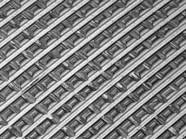
A first type of defect was simulated with black spray paint droplets, and a second type of defect was simulated by passing graphite powder through a screen. The workpieces were prepared and imaged with a Mitutoyo QVSTREAM machine vision inspection system at Micro Encoder, Inc.
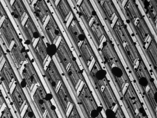
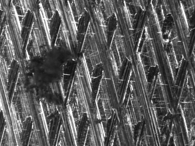
Aluminum workpiece with second type of defect.
For each set of images, I trained a Naïve Bayes model based on several preliminary treatments of the images. These treatments included raw images, second level Haar wavelet transformed images (only approximation coefficients), and first level Symlet 4 wavelet transformed images (including approximation coefficients, horizontal detail coefficients, vertical detail coefficients, and diagonal detail coefficients). I trained a Naïve Bayes model using training data that included both types of defects labeled as “defective” or “non-defective,” and using training data that included both types of defects labeled as “type 1 defective,” “type 2 defective,” or “non-defective.”
To compare machine learning techniques, I trained models using neural network classifiers trained on raw images for each type of defect individually, for combined defects labeled “defective” or “non-defective” (combined binary), and for both types of defects (three type) labeled as “type 1 defective,” “type 2 defective,” or “non-defective.” For the binary classifications I trained the networks with a simple single layer with different numbers of nodes, as well as a three layer network with a log-sigmoid transfer function, a linear transfer function, and a radial basis transfer function. I only used a single layer for the combined binary and the three type since the three layer did not give any significant advantage when I tested the individual defect models.
I cross validated each method by training a new model 20 times (with the same parameters) and calculated the overall average accuracy over the 20 trials.