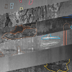
I did another Kaggle challenge in March. This was for a contest from Severstal Steel for detecting manufacturing defects in images of steel. There was a massive $100,000 collection of prizes. I entered the contest late and had no expectations of winning. By the time I had a testable model together the contest was over, but I was going for education, and not expecting a prize for this contest.

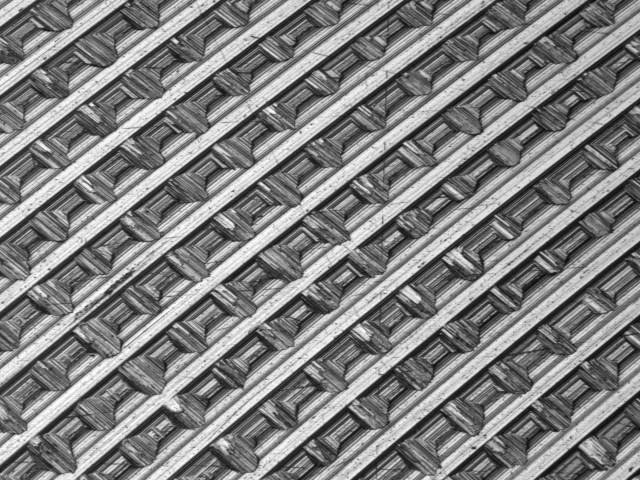
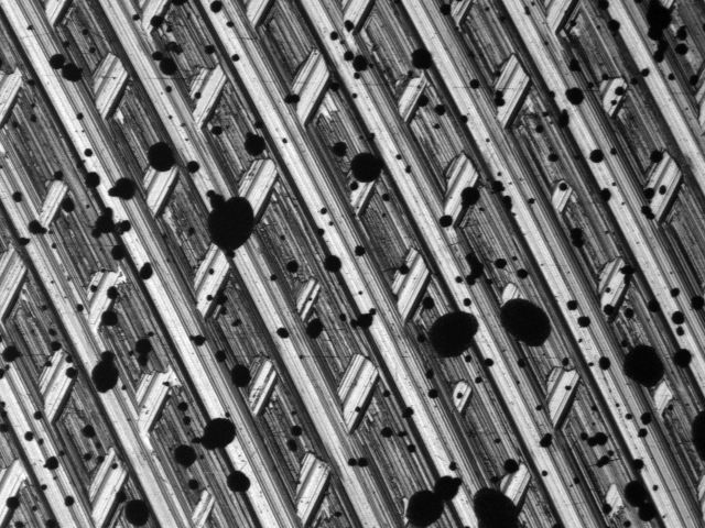
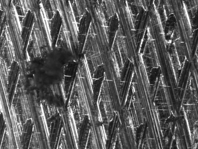
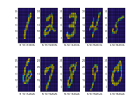
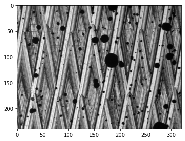
I had previously been working on a UNet model for detecting defects on aluminum workpieces, based on a data set from my previous job at Micro Encoder. This set included two types of simulated defects, one made with black spraypaint droplets, and one with graphite passed through a screen, as well as a pixel mask for the defect in each image. I was able to construct a very successful segmentation model that could detect either type of defect in an image and provide a corresponding pixel mask. I used a rather simple UNet architecture that would output two segmentation masks corresponding to each class of defect. Some sample images are below.

• 

• 

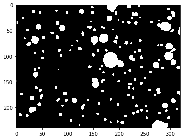
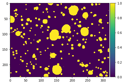
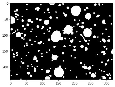
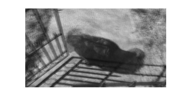
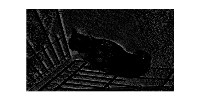
Examples of a pixel mask that my model predicted (left) and the actual pixel mask (right).

The Kaggle data set was a bit more complicated. There were four types of defects and unlike the earlier data set, some images included more than one type of defect. I used a similar approach with images downsampled by various scale factors, but my UNet model did not give very good results as measured by a Dice coefficient. I then tried using transfer learning using the Keras segmentation-models library with a ResNet34 backbone . I trained on a subset of data that included an equal number of images from each class of defect. I also added some augmented images with horizontal flips and vertical flips. When I used images downsampled by a scale factor of 2 (i.e. to 800×128), it bumped me above 0.80 for the dice coefficient. I then tried using an ensemble of models to improve accuracy. I used three UNet models with backbones including ResNet34, DenseNet121, and Inception. This gave me a dice coefficient of about 0.84. The winning submissions for the contests were around 0.90 for the dice coefficient. I hope to improve to something even closer to that.

I am now working on an improved model which uses a data pipeline with a data generator class rather than just a big numpy array, so I can avoid memory problems with large training data sets. I am also using more augmentation such as zoom and rotations. I hope to have some results soon.

I took part in a Kaggle challenge presented by Bengali AI.  The goal of this challenge is to build a machine learning model to identify images of handwritten Bengali graphemes, thus improving the state of the art for Bengali optical character recognition.  Each grapheme has three parts: a grapheme root, a vowel diacritic, and a consonant diacritic.  The grapheme root is one of 168 classes, the vowel diacritic is one of 11 classes, and the consonant diacritic is one of 7 classes.  The training set provided by Bengali.ai includes 200,840 images.  Kaggle ranked the entries by computing the fraction of all of the predictions (three per image) over a test set of about 200,000 images.  In my opinion, it would be a better metric to compute the fraction based on the graphemes as a whole, that is, where all three components of an image must be correct to count as a correct answer.  Optical character recognition of an abugida script such as Bengali should recognize the entire grapheme, not just the parts. The accuracy of the contest entries would be considerably lower if all three parts were considered for each grapheme.

I used several approaches of convolutional neural networks.  I started with transfer learning with a DenseNet121 model followed by two dense layers.  The final layer was split into three components for each of the three grapheme parts, such that the model output predictions in the form of a list of length 3.  This gave me an accuracy of 93.7%.  Then, I tried a similarly constructed MobileNet model.  This gave me an accuracy of 94.4%.  Finally, I tried an ensemble of both models, i.e. using an average of the probabilities from the predictions of both models to make a final prediction.  This gave me an accuracy of 95.3%. 

I was late to this contest, so I was not a contender for the prize.  The prize had already been awarded, but I chose to do the challenge as a learning experience to improve my skills.

I built my models using Keras, and included a few pieces of code forked from a public kernel on Kaggle for image resizing.  I used data augmentation with the Keras ImageDataGenerator class, including random rotations, horizontal shifts, and zoom.

As would be expected, the grapheme root was the most difficult part to predict because it included 168 classes.  The classes were highly imbalanced, with some of the majority classes over 100 times more frequent than the minority classes.  Class balancing weights might improve the model.  I will also try implementing the new AdamW optimizer.  This is similar to the beloved Adam optimizer, but with a decaying weight attached to the L2 component of the optimization algorithm.  I also plan to try one or more additional models as standalone models, and as parts of an ensemble.

As a two stage project, my final project for two applied math classes included machine learning for identifying metal manufacturing defects. For the first stage, I used Naïve Bayes classification models to identify manufacturing defects on multiple types of workpieces. The first type included two variations of simulated defects on machined aluminum. The second type included defective integrated circuit leads.

A full paper describing the first stage of the project is here.

For the second stage, I used neural networks to identify manufacturing defects on machined aluminum. I presented the results of both stages as a poster presentation at the Physics Informed Machine Learning Workshop in June of 2019.

A copy of my poster is here.

A first type of defect was simulated with black spray paint droplets, and a second type of defect was simulated by passing graphite powder through a screen.  The workpieces were prepared and imaged with a Mitutoyo QVSTREAM machine vision inspection system at Micro Encoder, Inc.

For each set of images, I trained a Naïve Bayes model based on several preliminary treatments of the images.  These treatments included raw images, second level Haar wavelet transformed images (only approximation coefficients), and first level Symlet 4 wavelet transformed images (including approximation coefficients, horizontal detail coefficients, vertical detail coefficients, and diagonal detail coefficients).  I trained a Naïve Bayes model using training data that included both types of defects labeled as “defective” or “non-defective,” and using training data that included both types of defects labeled as “type 1 defective,” “type 2 defective,” or “non-defective.”

To compare machine learning techniques, I trained models using neural network classifiers trained on raw images for each type of defect individually, for combined defects labeled “defective” or “non-defective” (combined binary), and for both types of defects (three type) labeled as “type 1 defective,” “type 2 defective,” or “non-defective.” For the binary classifications I trained the networks with a simple single layer with different numbers of nodes, as well as a three layer network with a log-sigmoid transfer function, a linear transfer function, and a radial basis transfer function.  I only used a single layer for the combined binary and the three type since the three layer did not give any significant advantage when I tested the individual defect models.

I cross validated each method by training a new model 20 times (with the same parameters) and calculated the overall average accuracy over the 20 trials.

I used neural networks to determine time stepping evolution of dynamic systems given an initial condition. I trained the neural networks with differential equations solved with MATLAB’s ode45 solver for multiple random initial conditions.

The full paper describing this project is here.

Neural Networks are a useful tool for determining the evolution of dynamic systems based on a set of training trajectories and then providing the neural network with an initial condition. For this exercise, we used known differential equations which we solved with numerical tools to compare the performance of neural network models. In general, neural networks are useful to model dynamics for systems in which the governing equations are unknown and actual measurements are the only way to compare a model to a dynamic system.

The systems include a lambda-omega reaction-diffusion (RD) system, a Kuramoto-Sivashinsky (KS) system, and a Lorenz system.

For the first part, I used linear fitting to a library of functions to derive a system of two first order differential equations that characterize snowshoe hare and lynx population data over a period of 30 years. I compared various models of linear fittings using Kullback–Leibler (KL) Divergence, the Akaike Information Criterion (AIC), and the Bayesian Information Criterion (BIC). For the second part, I used linear fitting to a library of functions to derive a partial differential equation that characterizes video of a Belousov-Zhabotinsky Chemical oscillator. I compared various models using KL Divergence.

The full paper describing this project is here.

I used Dynamic Mode Decomposition (DMD) to analyze three videos, and to separate those videos into foreground and background frame data.

The full paper describing this project is here.

I selected three videos to explore Dynamic Mode Decomposition and to visualize the foreground and background frame data and the combination of the two. The first video was a cat by a gate. The second video was monarch butterflies with a sky background. The third video was monarch butterflies on a forest floor. Each video was 1980×1080 resolution. The first video was 30 fps. The second and third videos were 60 fps.

I used Gabor filters to generate spectrograms of audio data.  For the first part, I analyzed 9 seconds of the opening of Handel’s messiah using various window widths, window types, and translation step sizes and compared the results.  For the second part, I analyzed a recording of the song “Mary Had a Little Lamb” as played by piano and as played by a recorder.  For each recording, I generated a spectrogram and used the data from the spectrogram to derive a sheet music representation.

The full paper describing this project is here.

Gabor filtering provides a useful means to generate time varying spectrograms of time varying signals such as audio signals.  The Gabor uncertainty limit demonstrates the tradeoff between high resolution in the time domain and high resolution in the frequency domain.

For the first part, the initial data was a MATLAB file in the form of a one-dimensional array of 73,133 values sampled at a rate of 8,192 Hz over a total duration of 8.928 s.  I defined set of n=73,133 Fourier modes.  I scaled the wavenumbers by a factor of  for the FFT calculations, where L was then length of the audio data in seconds.  For each spectrogram, I defined a Gaussian window, a Mexican hat window, and a rectangular window, and for each window, I generated a spectrogram for three values of the translation step.

For the second part, the initial data included two wav files, one with a piano sampled at a rate of 43,840 Hz over a total duration of 16 s and one with a recorder sampled at a rate of 44,837 Hz over 14 s.  For each audio file, I generated spectrograms using a Gabor transform with a Gaussian window to analyze the frequency content to identify the fundamental frequencies of each instrument for each note of the song, and from this information, I generated a sheet music representation of the song.

For this project I used Principal Component Analysis (PCA) to analyze three sets of video frames of a moving mass under four different conditions: an ideal case, a noisy case, a case with horizontal motion, and a case with horizontal motion and rotation.

The full paper describing this project is here.

PCA is one of the most useful applications of Singular Value Decomposition (SVD).  For this experiment, I analyzed three videos of four cases of motion of a paint can mass on a spring.  The first case was an ideal case with only vertical motion.  The second case included a significant amount of noise in the videos due to camera shake.  The third case included horizontal motion, i.e. one more degree of freedom in motion compared to the ideal case.  The fourth case included horizontal motion and rotational motion, i.e. two more degrees of freedom in motion compared to the ideal case.

For each of the four cases, I started by applying a motion tracking algorithm to each set of video frames in order to find a centroid of the paint can object.  I synchronized the relative motion of the video frames by finding a minimum of the y displacement.  I then determined respective vectors representing the pixel positions (x,y) of the centroid of the paint can as measured by each of the three cameras denoted a, b, and c.  From these respective vectors, I generated the final matrix X and applied SVD to the matrix X in order to determine the principal components of the motion.

I used five different methods of linear fitting to map images of hand drawn digits: LASSO, robustfit (least squares), QR decomposition, Moore-Penrose pseudoinverse, and ridge regression.  I compared the characteristics of each fit.  For each method, I also determined the pixels which represented 90% of the total pixel weightings (summed over each image), and created a sparse fit.  I then determined the pixels which represented 90% of the total pixel weightings for each individual digit and created a sparse fit.

The full paper describing this project is here.

The hand drawn digits came from the MNIST training data set which includes 60,000 labeled images of hand drawn digits 0 through 9.

QR Decomposition and pinv gave the highest accuracy (percentage true) results for the full fit, but gave very poor accuracy for the sparse fits.  Robustfit gave the best sparsity to produce comparable accuracy, especially for the individual digit pixel masks.  Ridges required by far the most pixels for 90% of the weightings.  Robustfit only required 87 pixels, whereas ridges required 4638.  However, ridges gave much better accuracy.  Using individual digit pixel masks generally gave better accuracy.

One of my Spring courses was a course taught in C++ teaching the basics of high performance computing. We learned how to build a linear algebra solver with customized vector and matrix classes that we then applied to solving partial differential equations. We used benchmarking to quantify different ways of improving performance of linear algebra operations.

First, we constructed the vector and matrix classes, including addition and multiplication operators. We tested different means of doing matrix and vector multiplication, e.g. different ordering for processing the products in order to take advantage of processor cache and SIMD vectorization. We compared the performance of different types of memory storage including row ordered and column ordered matrices.

Next, we created sparse matrix classes including coordinate ordered, compressed sparse row, and compressed sparse column matrices, and compared their relative performance.

Next, we focused on parallel programming. First, we created threads manually, then we used OpenMP and various types of pragma statements. We emphasized techniques for avoiding race conditions. We tested our operations using an Amazon Web Services account.

Next, we focused on GPU programming, more specifically, on CUDA programming. We tested our operations on a Tesla GPU server.

Finally, we focused on Message Passing Interface (MPI) programming. We tested our operations with up to 16 nodes. As our culmination of our work, we applied our matrix and vector classes to solving partial differential equations.